(-0.0014073334+0.99473155X+4.3362376E-4X2-0.15732671X3-2.94885E-5X4+0.0057283673X5)/(1.0),
where X=x1.0

Given and calculated data:
| Examples |
|
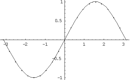
Example 1. Initial data, which were subject to approximation, were generated by the function sin(x) with changing values of its argument on the interval [-π , π] with the step π/10. This example contains data with positive and negative values; corresponding curve has maximum and minimum. These data are not good for fitting, however we reached perfect approximation of them when the number of coefficients of Pade function was equal to 6.
Input file contained coordinates of 21 points:
|
| Output: |

| x-coordinates | Given y-coordinates | Calculated y-coordinates |
| -3.1415 | 0.0 | -2.220446E-16 |
| -2.82735 | -0.309008 | -0.29142043 |
| -2.5132 | -0.58777 | -0.57676625 |
| -2.19905 | -0.809001 | -0.809001 |
| -1.8849 | -0.951045 | -0.95792145 |
| -1.57075 | -1.0 | -1.008054 |
| -1.2566 | -0.951045 | -0.9565521 |
| -0.94245 | -0.809001 | -0.8110919 |
| -0.6283 | -0.58777 | -0.58777 |
| -0.31415 | -0.309008 | -0.3089996 |
| 0.0 | 0.0 | -0.0014073334 |
| 0.31415 | 0.309008 | 0.30626994 |
| 0.6283 | 0.58777 | 0.5852885 |
| 0.94245 | 0.809001 | 0.809001 |
| 1.2566 | 0.951045 | 0.95495975 |
| 1.57075 | 1.0 | 1.0070201 |
| 1.8849 | 0.951045 | 0.9574435 |
| 2.19905 | 0.809001 | 0.809001 |
| 2.5132 | 0.58777 | 0.57707644 |
| 2.82735 | 0.309008 | 0.29176965 |
| 3.1415 | 0.0 | -6.661338E-16 |
|
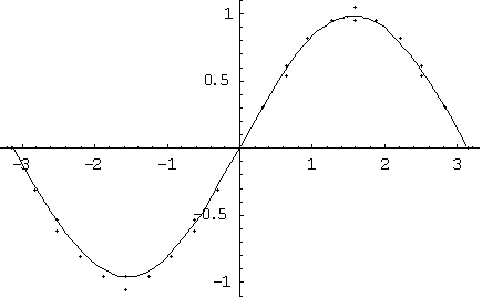
Example 2. This example shows the possibility of fitting of experimental data with dispersion. For instance there are two points with the same abscise equal to -2.5132 in this example. The corresponding values of function are -0.55777 and -0.61777. The mean value is -0.58777, which exactly corresponds to the value in the previous example. There are also several similar points at x= -1.57075; -0.6283; 0.6283; 1.57075; 2.5132.
Input file contained coordinates of 27 points: When the number of coefficients of Pade function was equal to 8, we almost reached the accuracy of approximation corresponding to the initial accuracy of entered data, because in this case we have obtained that 'Number of iterations without significant changing of correlation coefficient is 2'.
|
| Output: |

Given and calculated data:
| x-coordinates | Given y-coordinates | Calculated y-coordinates |
| -3.1415 | 0.0 | 0.0 |
| -2.82735 | -0.309008 | -0.29043132 |
| -2.5132 | -0.55777 | -0.536537 |
| -2.5132 | -0.61777 | -0.536537 |
| -2.19905 | -0.809001 | -0.72719085 |
| -1.8849 | -0.951045 | -0.8509647 |
| -1.57075 | -1.05 | -0.8976465 |
| -1.57075 | -0.95 | -0.8976465 |
| -1.2566 | -0.951045 | -0.8604723 |
| -0.94245 | -0.809001 | -0.73883086 |
| -0.6283 | -0.55777 | -0.54076564 |
| -0.6283 | -0.61777 | -0.54076564 |
| -0.31415 | -0.309008 | -0.28422365 |
| 0.0 | 0.0 | 0.003972023 |
| 0.31415 | 0.309008 | 0.29174328 |
| 0.6283 | 0.55777 | 0.54711586 |
| 0.6283 | 0.61777 | 0.54711586 |
| 0.94245 | 0.809001 | 0.74353784 |
| 1.2566 | 0.951045 | 0.8634039 |
| 1.57075 | 1.05 | 0.8989805 |
| 1.57075 | 0.95 | 0.8989805 |
| 1.8849 | 0.951045 | 0.85109234 |
| 2.19905 | 0.809001 | 0.7266036 |
| 2.5132 | 0.55777 | 0.53573227 |
| 2.5132 | 0.61777 | 0.53573227 |
| 2.82735 | 0.309008 | 0.2898508 |
| 3.1415 | 0.0 | 0.0 |

Given and calculated data:
| x-coordinates | Given y-coordinates | Calculated y-coordinates |
| -3.1415 | 0.0 | 0.0 |
| -2.82735 | -0.309008 | -0.29323664 |
| -2.5132 | -0.55777 | -0.56196564 |
| -2.5132 | -0.61777 | -0.56196564 |
| -2.19905 | -0.809001 | -0.778094 |
| -1.8849 | -0.951045 | -0.91780293 |
| -1.57075 | -1.05 | -0.9658279 |
| -1.57075 | -0.95 | -0.9658279 |
| -1.2566 | -0.951045 | -0.9175352 |
| -0.94245 | -0.809001 | -0.7786925 |
| -0.6283 | -0.55777 | -0.563773 |
| -0.6283 | -0.61777 | -0.563773 |
| -0.31415 | -0.309008 | -0.29382867 |
| 0.0 | 0.0 | 0.0054662297 |
| 0.31415 | 0.309008 | 0.3056081 |
| 0.6283 | 0.55777 | 0.57728875 |
| 0.6283 | 0.61777 | 0.57728875 |
| 0.94245 | 0.809001 | 0.7930391 |
| 1.2566 | 0.951045 | 0.9304703 |
| 1.57075 | 1.05 | 0.975482 |
| 1.57075 | 0.95 | 0.975482 |
| 1.8849 | 0.951045 | 0.92438054 |
| 2.19905 | 0.809001 | 0.78398645 |
| 2.5132 | 0.55777 | 0.56954676 |
| 2.5132 | 0.61777 | 0.56954676 |
| 2.82735 | 0.309008 | 0.3011712 |
| 3.1415 | 0.0 | -3.2727079E-15 |
|
Example 3. In this example the 'exact solution' of fitting problem is function 1/x0.5. Data were generated by this function on the interval [0.1; 100].
Input file contained coordinates of 7 points: We reached the exact solution at the first step of approximation. The obtained formula can be easily simplified.
|
| Output: |
Given and calculated data:
| x-coordinates | Given y-coordinates | Calculated y-coordinates |
| 0.01 | 10.0 | 10.0 |
| 0.16 | 2.5 | 2.5 |
| 0.25 | 2.0 | 2.0 |
| 1.0 | 1.0 | 1.0 |
| 4.0 | 0.5 | 0.5 |
| 25.0 | 0.2 | 0.2 |
| 100.0 | 0.1 | 0.1 |